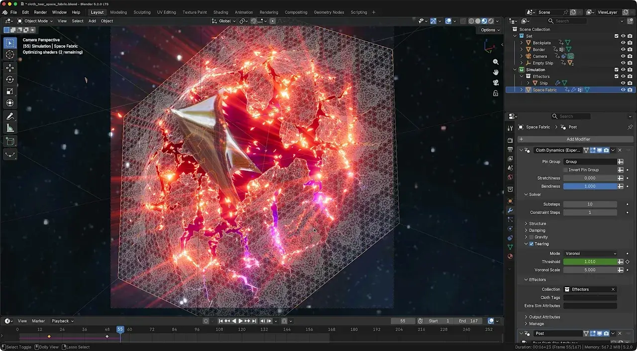
In the official demo file, a sheet of "space fabric" ends up ripped into two stiff panels, frozen against the dark.18 Cloth falling in a 3D package is nothing new. The interesting part sits elsewhere: that tear does not come from some tearing-strength slider buried in a panel. It comes from a node graph anyone can open, read and modify, constraint by constraint.
All of it arrived quietly with Blender 5.2 LTS on July 14, 2026.3 The new cloth and hair dynamics, still flagged experimental, are no longer sealed systems bolted onto the side of the application. They are node groups built on top of a new built-in physics solver, the XPBD Solver, itself available inside Geometry Nodes.12 On July 30, Jacques Lucke, one of the developers at the center of this work, published a post spelling out where it leads: interchangeable solvers, physics available everywhere including sculpt mode, and room for existing third-party libraries.1
For artists it fits in one sentence: the physics of your shot stops being a black box and becomes material you can take apart. For the open source ecosystem, it is an architectural decision, and those deserve a close look.
One box too many
History explains why this shift matters. For years, Blender's physics lived in separate compartments, each with its own panels and internal rules. The particle system handled hair and swarms. Cloth had its dedicated modifier. Fluids and smoke were replaced wholesale in 2020 by Mantaflow, which arrived with version 2.82.15 Rigid bodies ran on Bullet, an external library that entered through the game engine door back around Blender 2.42 before equipping the animation scene a few years later.17
Each system worked; some worked very well. But none was designed to be opened. You picked options in an interface: stiffness, damping, collisions. Under the hood, nothing invited an artist to read how motion was computed, or a third-party contributor to plug in their own solver. And the systems barely spoke to each other: getting a garment, hair and debris to interact cleanly took jury-rigging.
Meanwhile another part of Blender was changing philosophy. Geometry Nodes, launched in late 2020, turned modeling into visual programming. Simulation zones, introduced with 3.6 in 2023, already let the result of one frame feed the next, so you could write small homemade simulations in nodes.16 What was missing was the centerpiece: a real physics solver, fast and general enough, sitting directly inside the graph. That is exactly what 5.2 delivers.
Constraints, not forces
The technical core carries a lab-sounding name: XPBD, extended position-based dynamics. The method descends from well-identified research. In 2006, Matthias Müller and colleagues published Position Based Dynamics: instead of computing forces and integrating accelerations, you directly manipulate point positions to satisfy constraints, like "this edge keeps its length".6 A decade later, Macklin, Müller and Chentanez added the missing piece, compliance, which lets a constraint be soft rather than rigid. XPBD was born, presented at the Motion in Games conference in 2016.5
Why did this family of methods conquer visual effects? It trades physical exactness for what artists actually ask for: stability even at large time steps, direct control over results, and speed of setup. Blender's documentation says it plainly: geometry points are simulated as point masses under gravity, wind and collisions, held together by structural constraints like edge length and bending.4 In this model, cloth is just a mesh whose edges refuse to stretch and whose faces refuse to fold too fast.
The choice is not exotic. Houdini, the reference tool for VFX studios, runs its Vellum system, used for cloth, hair, grains and soft bodies, on an approach SideFX explicitly describes as extended position based dynamics.13 Since Houdini 19 in 2021, Vellum has also covered fluids and rigid bodies with the same algorithms.14 Blender is not taking a risky bet here: it adopts a production-proven method and makes it public, down to the last node.
That softness is not paint slapped over the math; it is part of the math. XPBD replaces stiffness with its inverse, compliance, and solving produces for each constraint a Lagrange multiplier that reads as a force: newtons for an edge length, newton-meters for a rotational torque.4 When an artist softens a cloth, the bundled node groups translate the intuitive softness value into physically correct compliance, in the documentation's own words.4 The panel slider and the paper's equation tell the same story, which is far from always true in computer graphics.
A node named solver
Concretely, 5.2 ships a built-in node named XPBD Solver. It looks unlike any classic physics panel: its main input is called World, and it takes a bundle of typed data containing the geometry to simulate, the constraint declarations targeting it, and outside effectors such as damping or collision.4 On the output side, the same bundle comes back with positions, rotations and velocities updated after one time step.
The internals are documented in unusual depth for a consumer solver. At each step, the node integrates velocities, advances positions, detects contacts, solves constraints with an iterative Gauss-Seidel method, recomputes velocities from corrected positions, then applies friction and damping.4 The step can be split into interpolated substeps for stability, including for animated colliders that deform over time. The solver even outputs a residual error measurement: above 1, the documentation recommends raising the iteration count. A solver that tells you when it solved badly — a genuinely useful idea.
The data flowing through is readable. Geometry carries named attributes: position, velocity, mass, and for rotations a quaternion, an angular velocity, a moment of inertia.4 Constraints themselves become attributes too, named through an explicit scheme that says which bundle they come from. In other words, a cloth stiffness value is no longer a cursor locked inside a modifier: it is a per-point field you can paint, modulate, animate. The documentation shows the example of hair stiffness strong at the root falling off toward the tips.
Hair as Cosserat rods
Hair shows how far the method stretches. Simulating a curl requires handling torsion as much as bending, and classic beam models collapse there. The team chose the Cosserat rod model, which describes each curve segment by a position plus a material frame independent of the tangent, capable of bending, twisting and shearing.4 In practice two specialized constraints work in pairs: one prevents stretch and shear, the other links neighboring segments to preserve their rest rotation, the thing that gives stiff hair its shape and curls their bounce.
The fun detail: those per-segment rotations are an extension Blender brought to the original XPBD formulation, which only manipulated positions.4 The project is not just consuming academic literature; it extends it for its context, and documents the extension.
The anchoring itself deserves a look. The position of each curve's first point is fixed to a surface mesh point, and the first segment's rotation aligns with the normal, optionally keeping a rest angle: hair can grow at an angle, as it so often does.4 Nothing exotic technically, but everything is written down, named, reusable in another setup.
Limits remain, stated in plain text. No self-collision yet: different parts of the same cloth pass through each other, and the documentation explains why this is hard, depending on the simulated geometry type.4 Contact detection caps out at 60 meters per second of relative velocity, a single point may hold only one contact per collider, and the current cloth bending constraint is explicitly labeled a placeholder. The whole system stays experimental because the team refuses to lock a design before broad feedback.2 This is a serious foundation, not a finished product, and nobody at Blender claims otherwise.
Coloring for speed
A solver living inside Geometry Nodes shares compute time with everything else in the pipeline. The parallelization effort is documented, and its mechanics say a lot about what topology costs.4 Most steps of the cycle run in parallel across all points without trouble: external forces, integration, contact detection, final update. Difficulty arrives with constraints touching several variables at once. Two constraints pulling on the same point cannot be evaluated at the same time.
First trick: chunking. Geometry gets sliced into pieces, and purely local constraints, pinning, the structure of a single hair, stay confined to their slice. When all constraints are local, the entire time step runs in parallel with no synchronization at all. Otherwise the solver falls back to a greedy graph coloring algorithm: every constraint gets a color, two constraints sharing a variable never share one, and same-colored constraints evaluate together without any risk of overwriting each other.
Contact handling follows the same honesty. Every contact creates a temporary constraint, refreshed as contacts change from substep to substep. Friction distinguishes static from dynamic, with the textbook image that comes with it: a box on an inclined plane starts sliding once the angle passes the friction angle.4 Between geometry and collider, the combined coefficient is computed as the geometric mean of the two, a convention explicitly documented rather than buried in code.
Effectors à la carte
Around the solver, 5.2 also installs vocabulary that will matter later. One word first: effector. Anything influencing the simulation qualifies. Gravity and surface collision come built into the cloth and hair assets. Three customizable effector types exist already: a collider, accepting any closed mesh; a custom force, computing a force vector per point; and the custom effector, injecting arbitrary behavior at a chosen stage of the cycle through a closure.12
The closure deserves a second look. It lets graph code run at a chosen moment, say right after solving, with access to all geometry currently being simulated. That is the kind of hook that used to live in simulation frameworks reserved for well-equipped studios. Filters complete the picture: each simulated geometry can carry tags, and each effector declares which ones it affects. Two cloths in the same scene can obey two different gravities without duplicating systems.
The catalog is young, for that matter: beyond built-in gravity, no ready-made forces ship yet, and the documentation suggests building your own, including as force objects through the Set Effector node and the Geometry Nodes now accepted on Empty objects.12 An admitted gap with the good taste of pointing exactly where the community can already step in.
These bricks feel like a construction set, deliberately. High-level assets such as the Cloth Dynamics modifier are just node groups around the solver, intentionally hackable: the first documented customization path is adding or removing constraints inside those groups, the second is building an entirely new system directly on the XPBD Solver, harder because you must supply the typed bundles it expects.12 Between those two, a full spectrum of tinkering depths.
Physics as data
A second shift, quieter but just as structural, explains a lot: geometry bundles. Introduced in 5.0, bundles are packages of arbitrary data; 5.2 lets you attach them to geometry itself, carried across modifier boundaries and even object boundaries, fields and closures included.7 The May 2025 post on declarative systems showed where that leads: behaviors defined here, consumed there, with no implicit wiring.8
The new physics is the first major customer of that infrastructure. When the Capture Rest Geometry modifier records how a surface moved from rest to deformed state, those data travel in a bundle attached to the mesh, and the hair system reads them back further up the stack.2 An effector parked on an object gets found by the simulation because it was attached to geometry, not because a checkbox declared some global relationship.1
This point matters more than the solver itself. Solvers get replaced. A shared convention for how scenes carry their physics data organizes an entire ecosystem: tomorrow it should let two different solvers receive the same objects, the same tags, the same forces, simply because those things became standardized data rather than module internals.
A borrowed engine
The roadmap confirms the ambition, and borrowing is part of the plan. For fluids, work is ongoing: the first public piece is a pull request adding a Grid Solve Poisson node, which takes a scalar grid as input and solves the Poisson equation, the mathematical brick behind pressure and flow-map computation in fluid simulation.9 A detail worth noting: the PR author is Brady Johnston, a Scotland-based structural biologist known for creating Molecular Nodes, a bridge between molecular biology and Blender. Blender's physics is already being written by more than one pair of hands.
For rigid bodies, the post names Jolt, the library created by Jorrit Rouwe: multithreaded, deterministic, used by Horizon Forbidden West and Death Stranding 2.110 Blender has "started looking into it", mainly for solids. Godot's precedent hints at the path: the game engine integrated Jolt into version 4.4 in March 2025 after the community extension proved itself, with Jolt's creator helping on the bindings.11 An AAA engine born inside a PlayStation studio becoming an open source brick in two free creation tools: that scenario is no longer theoretical.
Why not write one giant in-house solver? The post answers plainly: "While a single physics solver that does everything would be perfect, it is unrealistic since each solver comes with trade-offs."1 Every method wins somewhere and loses somewhere else. The chosen strategy is a common framework where several engines coexist, some written internally, others taken from existing libraries, high-level assets picking the right solver for the right task. The December 2025 Nodes & Physics module meeting already lists replacing the old non-hair particle functionality and integrating Jolt for rigid bodies in Geometry Nodes on its agenda.12
Hands in the graph
What does this change for someone making images? The entry level, for starters, moves up: adding cloth to a mesh takes one modifier, with pinning, stretch and bend controls, and tearing built in.2 Hair goes through an operator that installs everything automatically, surface and constraints included. Early community work quoted on the official release page sets the tone: vegetation reacting to an animated hippo walking past, optimized cloth experiments, and this user comment that captures the spirit, "i learned a lot about the new cloth solver nodes".3
There is another very tangible effect: physics moves closer to the other gestures of making. The announced work on modal node tools should make solvers available for destructive editing, in edit and sculpt modes, and in interactive applications.1 Translation: push a drape by hand while it solves, sculpt against a running simulation, use physics as a modeling tool rather than only as a final calculation stage. Anyone who has nudged a frozen simulation cache blind can picture the practical gain.
And then there is the most interesting part here, for IRZ as much as for any curious mind: the very design of the system teaches something. Instead of locking simulation behind panels, Blender treats it like open code: constraints declared as data, a replaceable solver, documented extension points, limits stated honestly. A curious artist can climb from the torn cloth down to the edge that stopped holding. Closed simulation will never offer that traceability of gesture.
The subject remains young. The design may still move, self-collision is missing, and nothing guarantees every roadmap promise lands. But the direction is published and demonstrated, demo files included.18 Next time a cloth tears in your scene, the right question will no longer be "which parameter do I tweak?". It will be "which constraints do I want to open?".